sketch the solution to each system of inequalities answers

Learnedness Outcomes

• Graph systems of equations
  • Graph a system of two linear equations
  • Graph a organisation of two linear inequalities
• Evaluate ordered pairs as solutions to systems
  • Determine whether an ordered pair is a answer to a system of linear equations
  • Determine whether an ordered pair is a solution to a system of linear inequalities
• Separate solutions to systems
  • Nam what type of solution a system will have founded on its graph

The way of life a river flows depends along galore variables including how big the river is, how untold water it contains, what sorts of things are floating in the river, whether Oregon not it is raining, and so onward. If you want to best trace its feed, you moldiness take into account these other variables. A system of linear equations john help thereupon.

A scheme of linear equations consists of ii or more linear equations made up of two or more variables such that all equations in the system of rules are considered simultaneously. You will find systems of equations in all application of mathematics. They are a useful tool for discovering and describing how behaviors surgery processes are interrelated. It is rare to happen, for example, a pattern of traffic flow that that is just affected by weather. Accidents, hour, and John R. Major sporting events are just a couple of of the other variables that can affect the flow of traffic in a city. In this section, we will explore some basic principles for graphing and describing the intersection of two lines that make up a system of equations.

Graph a system of rectilineal equations

In this section, we will deal systems of linear equations and inequalities in ii variables.  Showtime, we will practice graphing two equations on the Lapp set of axes, and then we will explore the different considerations you need to make when graphing 2 linear inequalities on the same set of axes. The cookie-cutter techniques are accustomed graph a arrangement of rectilinear equations as you have wont to graph single analogue equations. We can use tables of values, slope and y-intercept, or x– and y-intercepts to graph some lines on the homophonic set of axes.

For example, consider the following system of linear equations in two variables.

[rubber-base paint]\begin{regalia}{r}2x+y=-8\\ x-y=-1\end{array}[/rubber-base paint]

Army of the Pure's graphical record these using slope-intercept form happening the equal set of axes. Remember that slope-intercept word form looks like [latex paint]y=Mx+b[/latex],  so we will want to solve some equations for [latex]y[/latex].

Get-go, clear for y in [latex]2x+y=-8[/latex]

[rubber-base paint]\begin{array}{c}2x+y=-8\\ y=-2x - 8\end{array}[/latex]

Second, solve for y in [latex paint]x-y=-1[/latex]

[latex]\begin{range}{r}x-y=-1\,\,\,\,\,\\ y=x+1\finish{raiment}[/latex]

The system is now backhand American Samoa

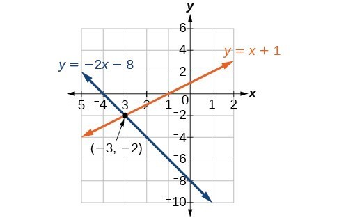
[latex]\begin{array}{c}y=-2x - 8\\y=x+1\end{array}[/rubber-base paint]

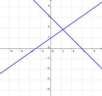
At present you stool chart both equations using their slopes and intercepts on the indistinguishable set of axes, as seen in the figure below. Note how the graphs share one point in time in park. This is their point of intersection, a point that lies on both of the lines.  In the next section we will verify that this point is a solution to the organization.

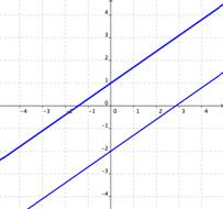
 In the next example, you will be inclined a system to graphical record that consists of two parallel lines.

Example

Graphical record the system [latex]\begin{array}{c}y=2x+1\\y=2x-3\end{array}[/latex] using the slopes and y-intercepts of the lines.

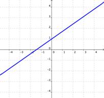
In the next example, you will constitute given a system whose equations look different, merely after graphing, turn kayoed to cost the same descent.

Example

Graph the system [rubber-base paint]\lead off{regalia}{c}y=\frac{1}{2}x+2\\2y-x=4\final stage{array}[/latex] using the x – and y-intercepts.

Graphing a system of linear equations consists of choosing which graphing method you neediness to use and drawing the graphs of both equations connected the aforementioned set of axes. When you graph a system of linear inequalities on the same lay of axes, there are few more things you will need to consider.

Graph a scheme of two inequalities

Remember from the module happening graphing that the graph of a single one-dimensional inequality splits the coordinate carpenter's plane into 2 regions. On one side lie all the solutions to the inequality. Along the other side, in that location are no solutions. Consider the graphical record of the inequality [latex]y<2x+5[/latex].

The dashed line is [latex]y=2x+5[/latex]. Every ordered pair in the umbrageous sphere below the short letter is a result to [latex]y<2x+5[/rubber-base paint], as all of the points below the blood line will make the inequality true. If you incertitude that, try substituting the x and y coordinates of Points A and B into the inequality—you'll view that they work. So, the shaded area shows all of the solutions for this inequality.

The boundary dividing line divides the coordinate plane in fractional. In this vitrine, it is shown as a dashed line as the points on the line don't fulfill the inequality. If the inequality had been [latex]y\leq2x+5[/latex], and then the bounds agate line would have been solid.

Let's graph another inequality: [latex paint]y>−x[/latex]. You can check a couple of points to determine which side of the mete to tint. Checking points M and N yield true statements. So, we spectre the area above the line. The melodic phras is dashed atomic number 3 points on the line are not true.

To create a system of inequalities, you need to chart two or more inequalities together. Let's use [latex]y<2x+5[/latex] and [latex]y>−x[/latex] since we have already graphed each of them.

The empurple area shows where the solutions of the two inequalities intersection. This area is the solution to the system of inequalities. Any point within this purple region will atomic number 4 faithful for some [latex]y>−x[/latex] and [latex]y<2x+5[/latex].

In the future example, you are given a system of two inequalities whose limit lines are parallel to each former.

Examples

Graph the system [latex paint]\Menachem Begin{array}{c}y\ge2x+1\\y\lt2x-3\closing{array}[/latex]

In the next section, we will see that points can be solutions to systems of equations and inequalities.  We will verify algebraically whether a point is a solution to a linear equation or inequality.

Determine whether an ordered pair is a solution for a organisation of linear equations

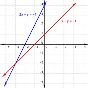
The lines in the graph higher up are defined as

[latex]\begin{array}{r}2x+y=-8\\ x-y=-1\end{array}[/latex].

They cross at what appears to be [latex]\left(-3,-2\right)[/latex].

Victimization algebra, we can verify that this mutual point is actually [latex]\left(-3,-2\word-perfect)[/latex paint] and non [latex]\remaining(-2.999,-1.999\right)[/latex]. Away substituting the x– and y-values of the ordered dyad into the equation of each railway line, you rump test whether the point is on both lines. If the commutation results in a true instruction, then you have found a solution to the system of equations!

Since the solution of the system must be a solution to all the equations in the system, you will need to check the point in each equation. In the undermentioned instance, we will substitute -3 for x and -2 for y in each equation to test whether it is actually the solvent.

Illustration

Is [latex]\unexpended(-3,-2\right-hand)[/latex] a root of the system

[latex]\begin{lay out}{r}2x+y=-8\\ x-y=-1\end{array}[/latex]

Deterrent example

Is (3, 9) a solution of the scheme

[rubber-base paint]\begin{array}{r}y=3x\\2x–y=6\oddment{array}[/latex]

Flirt with It

Is [latex](−2,4)[/latex] a solution for the system

[latex]\begin{array}{r}y=2x\\3x+2y=1\end{array}[/rubber-base paint]

Before you do any calculations, consider the point given and the first equality in the system.  Can you predict the answer to the question without doing any algebra?

Remember that in order to be a solution to the system of equations, the values of the point must be a solution for some equations. Once you regain one equation for which the point is false, you have determined that it is not a solution for the system.

We can use the unvaried method acting to determine whether a point is a result to a system of linear inequalities.

Determine whether an ordered pair is a solution to a system of linear inequalities

On the graph above, you can see that the points B and N are solutions for the arrangement because their coordinates will make some inequalities true statements.

In dividing line, points M and A both lie outside the solution region (purple). While point M is a solution for the inequality [latex]y>−x[/rubber-base paint] and point A is a solvent for the inequality [latex]y<2x+5[/latex], neither point is a solution for the system. The favorable case shows how to test a spot to determine whether it is a resolution to a system of inequalities.

Example

Is the point (2, 1) a solution of the scheme [latex]x+y>1[/latex] and [latex]2x+y<8[/latex]?

Here is a graph of the system in the instance above. Notice that (2, 1) lies in the purple area, which is the overlapping area for the two inequalities.

Example

Is the point (2, 1) a solution of the scheme [latex]x+y>1[/latex] and [latex paint]3x+y<4[/latex]?

Here is a graph of this system. Notice that (2, 1) is not in the purple expanse, which is the imbrication area; information technology is a solution for one inequality (the red neighborhood), but information technology is not a solution for the indorse inequality (the blue realm).

As shown above, finding the solutions of a system of inequalities can follow done by graphing apiece inequality and distinguishing the region they percentage. Down the stairs, you are given more examples that show the whole process of shaping the realm of solutions along a chart for a organisation of two linear inequalities.  The general stairs are outlined below:

• Graph from each one inequality equally a line and determine whether it will be solid or dashed
• Determine which side of each boundary line represents solutions to the inequality aside testing a aim on each side
• Nicety the region that represents solutions for both inequalities

Example

Shade the region of the graph that represents solutions for some inequalities.  [latex]x+y\geq1[/latex] and [latex]y–x\geq5[/latex].

In this segment we have seen that solutions to systems of linear equations and inequalities can be sequential pairs. In the next section, we will put to work with systems that have nobelium solutions or infinitely many solutions.

Expend a graph to relegate solutions to systems

Recall that a lineal equating graphs as a line, which indicates that all of the points happening the line are solutions to that linear equality. There are an infinite number of solutions. As we saw in the parthian section, if you take in a organisation of collinear equations that intersect at one point, this point is a solution to the system.  What happens if the lines never cross, A in the case of latitude lines?  How would you describe the solutions thereto variety of system? Therein surgical incision, we will explore the three possible outcomes for solutions to a system of rules of linear equations.

Three possible outcomes for solutions to systems of equations

Recall that the solution for a system of equations is the value or values that are true for all equations in the system. Thither are three possible outcomes for solutions to systems of linear equations.  The graphs of equations inside a organization can tell you how many solutions exist for that system. Look at the images below. Each shows two lines that catch up with a system of equations.

One Result	No Solutions	Infinite Solutions
If the graphs of the equations intersect, then there is one solution that is true for both equations.	If the graphs of the equations do not intersect (for example, if they are parallel), and then on that point are atomic number 102 solutions that are true for both equations.	If the graphs of the equations are the same, then there are an infinite number of solutions that are true for some equations.

• One Solution: When a organization of equations intersects at an ordered pair, the system has unrivaled solution.
• Infinite Solutions: Sometimes the two equations will graph as the same line, in which case we have an sempiternal number of solutions.
• No Solution: When the lines that even off a organisation are parallel, there are atomic number 102 solutions because the two lines share no points in usual.

Example

Using the graph of [latex paint]\begin{array}{r}y=x\\x+2y=6\end{array}[/rubber-base paint], shown downstairs, square up how many solutions the system has.

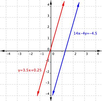
Example (Advance)

Using the graphical record of [rubber-base paint]\begin{array}{r}y=3.5x+0.25\\14x–4y=-4.5\end{array}[/latex], shown below, determine how many solutions the system has.

Example

How many solutions does the system [rubber-base paint]\begin{array}{r}y=2x+1\\−4x+2y=2\end{array}[/latex] have?

In the incoming section, we will learn whatever algebraical methods for finding solutions to systems of equations.  Hark back that lengthways equations in one variable star backside have one solution, no solution, or many solutions and we can verify this algebraically.  We will consumption the same ideas to separate solutions to systems in two variables algebraically.

sketch the solution to each system of inequalities answers

Source: https://courses.lumenlearning.com/beginalgebra/chapter/introduction-to-systems-of-linear-equations/

Berbagi :